6.3 Churn analysis
Estimating the risk of attrition related to each customer is an essential step to model the firm’s portfolio. In this context, survival models can be implemented with a view of deriving a predicted churn risk and survival function for each client. On the one hand, these predictions can be used to identify loyal consumers and make appropriate decisions. For instance, it might be relevant to offer benefits to a high-value client with a high estimated churn risk. On the other hand, a customer’s survival probability at time \(t\) represents the chance that this very customer be active in the portfolio at time \(t\). This measure is helpful to compute the estimated value of the portfolio in section 6.4.
Before presenting the estimation results, it seems important to recall that Tenure_Months and Churn_Value can be seen as a pair of time and event variables used as target in survival models.
| CustomerID | Tenure_Months | Churn_Value |
|---|---|---|
| 1671 | 30 | 1 |
| 6705 | 43 | 0 |
| 3702 | 12 | 0 |
| 1519 | 1 | 1 |
| 4882 | 50 | 0 |
6.3.1 The Cox model
When it comes to choose an estimation method on survival data, the Cox PH model appears to be an interesting first choice. As explained in chapter 3, this semi-parametric model makes no assumption regarding the nature of the baseline hazard function \(\lambda_0(t)\). The parametric part only relies in the modelling of the effect of some covariates on the hazard function \(\lambda(t)\) (see section 3.6.2 for more details).
Fitting the model on the selected features
Using the coxph function from the survival R library (Terry M. Therneau and Patricia M. Grambsch 2000), we are able to train a Cox model on the feature vector identified in section 6.1. Once the model fitted, it seems relevant to evaluate its performance on the train data set. Table 6.7 compares the model’s log-likelihood to the constrained model’s. Given the very low p-value, it can be assumed that the Cox model better fits the data than a model with only the intercept.
| Model | Constrained | pvalue | |
|---|---|---|---|
| -9228.77 | -10448.08 | 0 |
Concordance index \(c\) is another metric to assess the performance of models which produces risk scores. It is defined as the probability to well predict the order of event occurring time for any pair of instances (see section 3.8 for more details). For the Cox model, the C-index obtained on the training set is \(c \approx 0.865 \pm 0.004\), which is more than satisfying.
Marginal effects
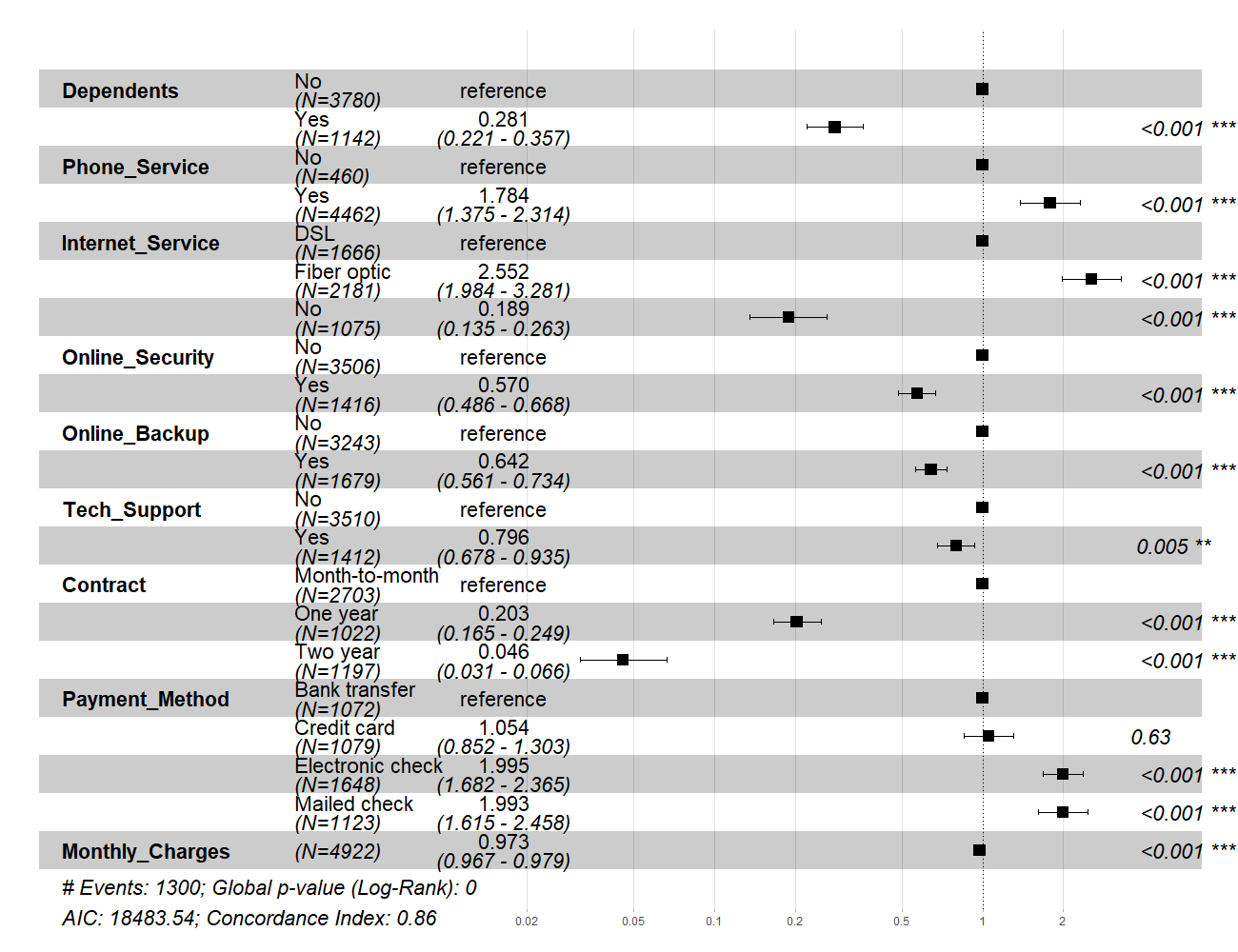
In the Cox model, the relative hazard between two observations is assumed to be constant over time. As a consequence, the relative hazard becomes \(\exp \hat{\beta}\) for both dummy and continuous variables. For instance regarding figure 6.7, the relative hazard ratio between customers with a two-year contract and those with a month-to-month contract is 0.046, meaning that the latter group is 22 times more prone to churn than the former. Also, month-to-month clients are about 5 times more likely to churn than customers enrolled in one-year plan. When analysing the relative hazard ratios related to the payment method, it comes that clients who pay by electronic or mailed check are two times riskier to churn than those who pay by bank transfer. Furthermore, being enrolled in a plan with additional services like Online_Security, Online_Backup or Tech_Support tends to decrease the estimated churn risk. As for the effect of the Internet_Service covariate on the risk of attrition, it seems to be mitigated since clients who have a fiber optic internet connection are more than twice as likely to churn as those using a DSL internet connection.
Figure 6.7: Marginal effects obtained with the Cox PH model

Estimation results
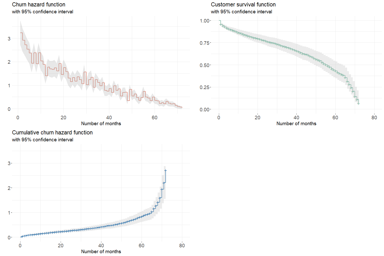
Semi-parametric models aims at estimating the instantaneous hazard function given a baseline hazard and a set of covariates. The model outputs a risk prediction for each individual with a confidence interval. Then, the survival and cumulative hazard functions can be retrieved as explained in section 3.3. When going deeper into the functions depicted in figure 6.8, it can be noticed some inconsistencies between the instantaneous hazard and cumulative hazard estimated functions. Given the cumulative churn hazard increases faster when the number of months is high and given the instantaneous churn hazard is supposed to be the cumulative hazard function’s slope, the estimated instantaneous hazard’s shape should be convex. One may deduce that the Cox model does not manage to properly estimate the risk of churn.
Figure 6.8: Aggregated churn hazard, survival and cumulative hazard functions estimated by Cox model

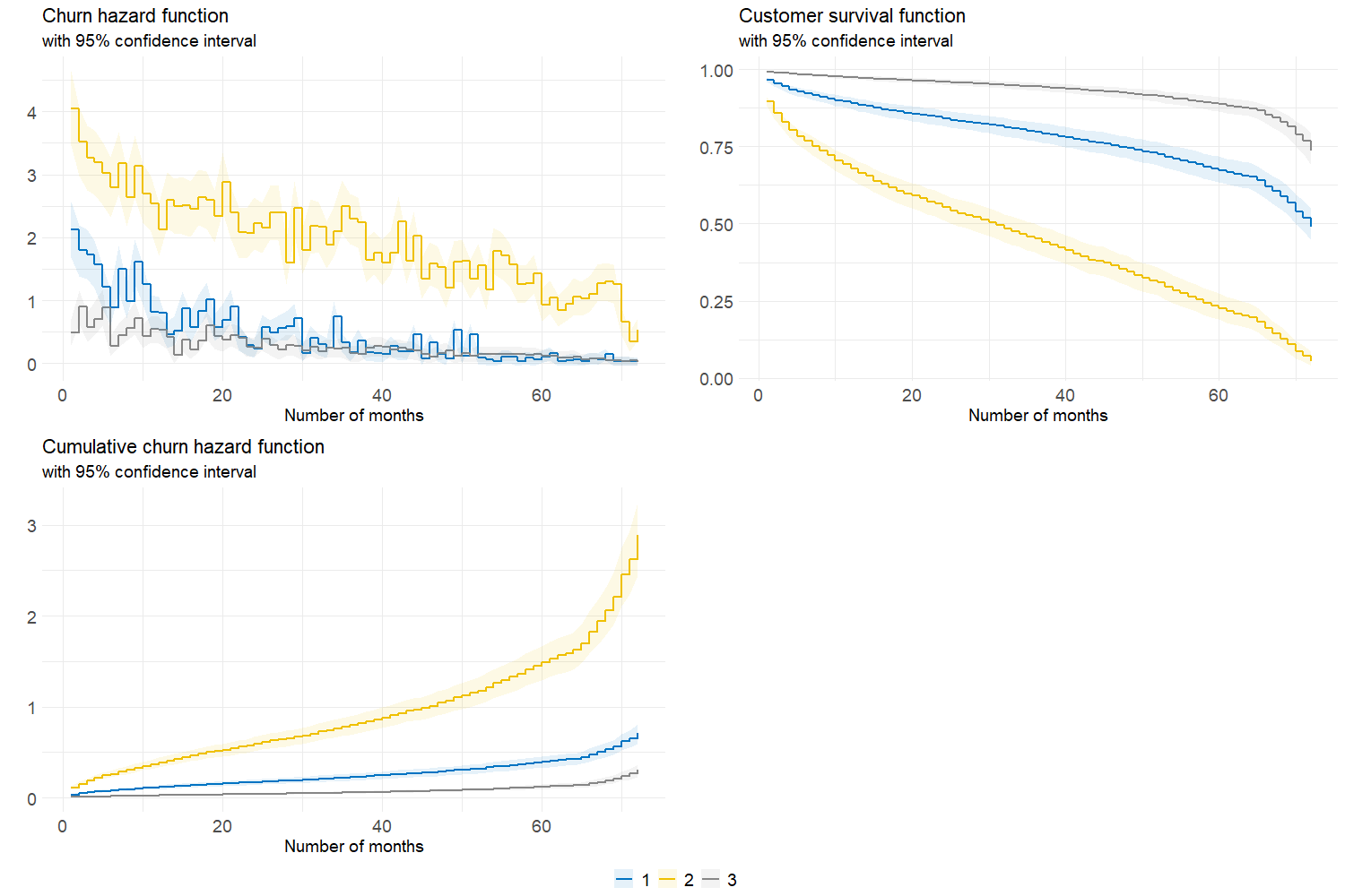
Although the fitted model is not flawless, it can be interesting to study the estimation differences between the 3 customer segments identified in the previous section. Looking at figure 6.9, one can conclude that Gold (cluster 2) clients are more prone to churn than others. Their aggregated risk of attrition is indeed higher to such an extent that the cumulative churn hazard is exploding when the number of months is greater than 60. This being said, an efficient portfolio management would be to find strategies to reduce Gold customers’ churn and increase their duration in the portfolio.
Figure 6.9: Aggregated churn hazard, survival and cumulative hazard functions for each cluster

6.3.2 Other survival models
As said in the previous part, the Cox model does not fit the data perfectly as it does not capture the churn hazard’s actual shape. In this context, it seems relevant to fit other survival models and test how they perform in predicting the risk of attrition. It is firstly decided to train parametric survival models which consist in assigning a probability distribution to the hazard function (see section 3.5 for more details). To that end, one can use flexsurv (Jackson 2016) which is and R package for parametric survival modelling. After having fitted the exponential, Weibull, gamma, log-logistic and log-normal models, no improvement can be observed with respect to the Cox model. Then, a machine learning approach can be adopted to model duration data using the random survival forest algorithm which is detailed in section 3.7. The rfsrc function from randomForestSRC (H. Ishwaran et al. 2008) is used to train the model after having determined the optimal node size and number of variables to try at each split with the tune function. Once the model trained, its performance is compared to the Cox model’s as shown by table 6.8. One cannot but admit that the random survival forest perform poorly in terms of concordance index with respect to the Cox model. The latter manages to output a better risk scoring than the ML algorithm.
| Train | Test | |
|---|---|---|
| Cox | 86.769 | 86.253 |
| RSF | 49.273 | 49.229 |
It is thus decided to select the Cox PH model for the rest of the study.