3.7 Machine Learning for Survival Data
In the previsous sections, some important models for duration data have been introduced. Here, emphasize is placed on machine learning algorithms that can also be implemented to predict a time-to-event variable such as the time to churn.
3.7.1 Survival Trees
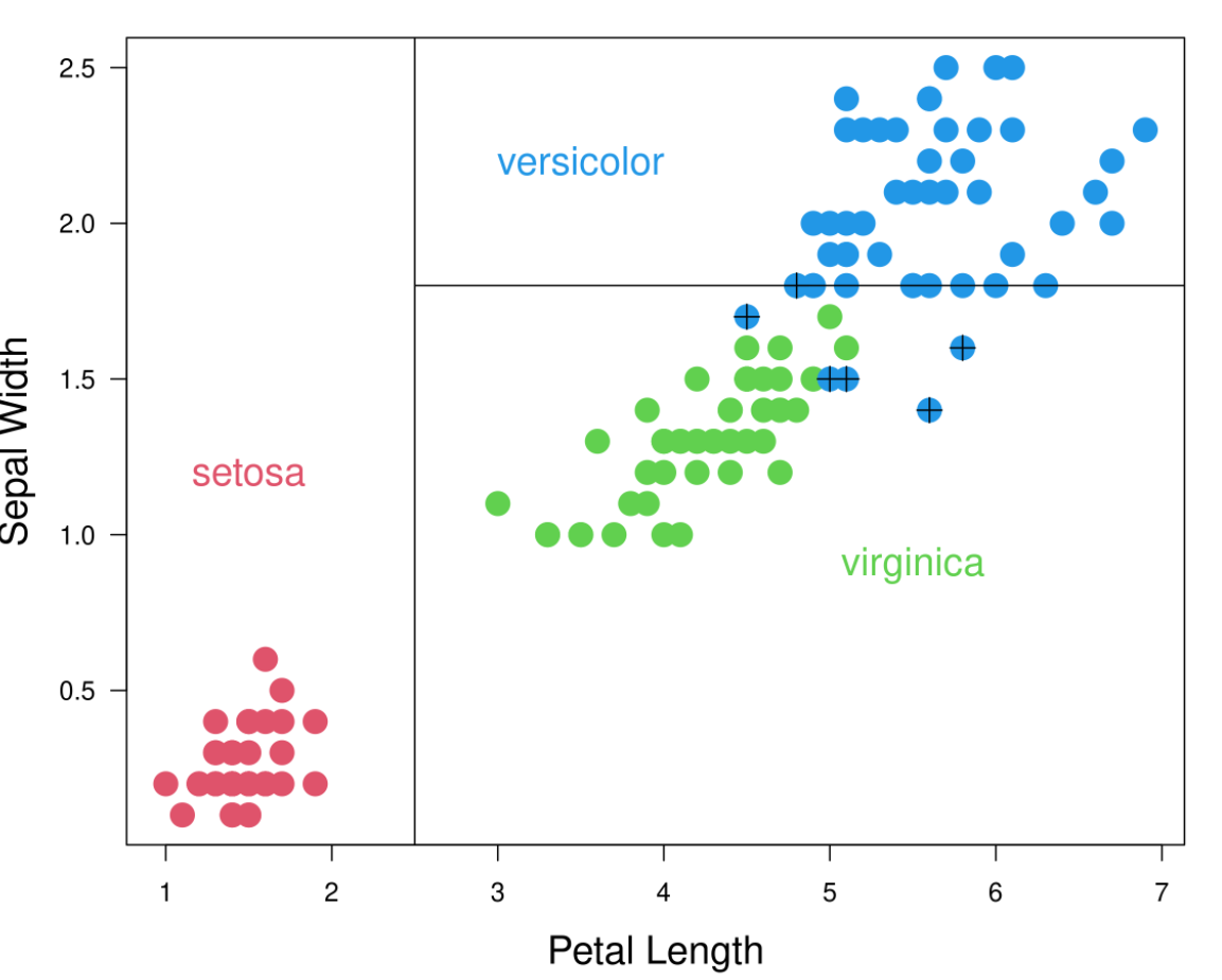
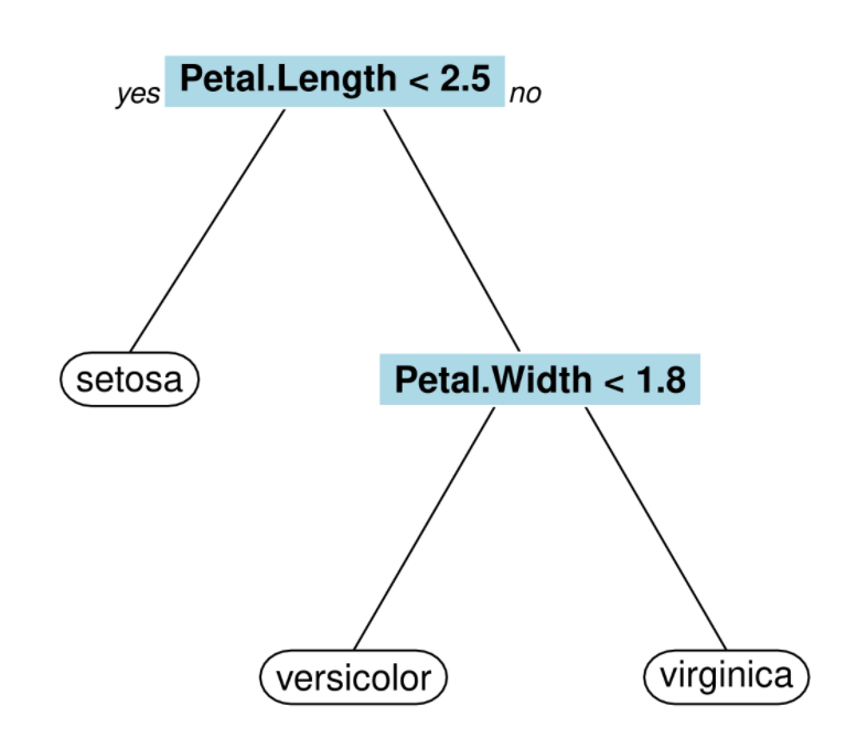
Traditional decision trees, also called CART (Classification And Regression Trees), segment the feature space into multiple rectangles and then fit a simple model to each of these subsets as shown by figure 3.5 (Scholler 2021b). The algorithm is a recursive partitioning which requires a criterion for choosing the best split, another criterion for deciding when to stop the splits and a rule for predicting the class of an observation.
Figure 3.5: Clasification decision tree


Survival tree (LeBlanc and Crowley 1993) is the adapted version of CART for duration data. The objective is to use tree based binary splitting algorithm in order to predict hazard rates. To that end, survival time and censoring status are introduced as response variables. The splitting criteria used for survival trees have the same purpose than the criteria used for CART that is to say maximizing between-node heterogeneity or minimizing within-node homogeneity. Nonetheless, node purity is different in the case of survival trees as a node is considered pure if all spells in that node have similar survival duration. The most common criterion is the logrank test statistic to compare the two groups formed by the children nodes. For each node, every possible split on each feature is being examined. The best split is the one maximizing the survival difference between two children nodes. The test statistic is \(\chi^2\) distributed which means the higher its value, the higher between-node variability so the better the split. Let \(t_1, \dots, t_k\) be the \(k\) ordered failure times. At the \(j^{\text{th}}\) failure time, the logrank statistic is expressed as (Segal 1988):
\[\begin{equation} \chi^2_{\text{logrank}} = \frac{\big[\sum_{j=1}^k \ (d_{0j} - r_{0j} \times d_j/r_j) \big]^2}{\sum_{j=1}^k \ \frac{r_{1j}r_{0j}d_j(r_j - d_j)}{r_j^2(r_j -1)}} \tag{3.20} \end{equation}\]
3.7.2 Random Survival Forests (RSF)
This algorithm is proposed by Hemant Ishwaran and al. (2011) and is an ensemble of decision trees for the analysis of right-censored survival data. As random forests used for regression and classification, RSF are based on bagging which implies that \(B\) bootstrap samples are drawn from the original data with 63\(\%\) of them in the bag data and the remaining part in the out-of-bag (OOB) data. For each bootstrap sample, a survival tree is grown based on \(p\) randomly selected features. Then, the parent node is split using the feature among the selected ones that maximizes survival difference between children nodes. Each tree is grown to full size and each terminal node needs to have no less than \(d_0\) unique events. The cumulative hazard function (CHF) is computed for each tree using the Nelson-Aalen estimator such as:
\[\begin{equation} \widehat{H_l}(t) = \sum_{t_{j, l} < t} \frac{d_{j,l}}{r_{j,l}} \tag{3.21} \end{equation}\]
where \(t_{j,l}\) is the \(j^{\text{th}}\) distinct event time in leaf \(l\), \(d_{j,l}\) the number of events completed at \(t_{j,l}\) and \(r_{j,l}\) the number of spells at risk at \(t_{j,l}\).
All the CHFs are then averaged to obtain the bootstrap ensemble CHF and prediction error is finally computed on the OOB ensemble CHF.
3.7.3 Cox Boosting
Boosting is an ensemble method which combines several weak predictors into a strong predictor. The idea of most boosting methods is to train predictors sequentially, each trying to correct its predecessor. Cox boosting (Binder and Schumacher 2008) is designed for high dimension survival data and has the purpose of feature selection while improving the performance of the standard Cox model. The key difference with gradient boosting is that Cox boosting does not update all coefficients at each boosting step, but only updates the coefficient that improves the overall fit the most. The loss function is a penalized version of the Cox model’s log-likelihood (see equation (3.19) for the likelihood function of the Cox model). Cox boosting helps measuring variable importance as the coefficients associated to more representative variables will be updated in early steps.